The dark arts of statistical genomics
“Whereof one cannot
speak, thereof one must be silent” - Wittgenstein
That’s a maxim to live by, or certainly to
blog by, but I am about to break it. Most of the time I try to write about
things I feel I have some understanding of (rightly or wrongly) or at least an
informed opinion on. But I am writing this post from a position of ignorance
and confusion.
I want to discuss a fairly esoteric and
technical statistical method recently applied in human genetics, which has
become quite influential. The results from recent studies using this approach have
a direct bearing on an important question – the genetic architecture of complex
diseases, such as schizophrenia and autism. And that, in turn, dramatically
affects how we conceptualise these disorders. But this discussion will also
touch on a much wider social issue in science, which is how highly specialised statistical
claims are accepted (or not) by biologists or clinicians, the vast majority of
whom are unable to evaluate the methodology.
Speak for yourself, you say! Well, that is
exactly what I am doing.

The technique in question is known as Genome-wide Complex Trait Analysis (or GCTA). It is based on methods developed in animal
breeding, which are designed to measure the “breeding quality” of an animal
using genetic markers, without necessarily knowing which markers are really
linked to the trait(s) in question. The method simply uses molecular markers across
the genome to determine how closely an animal is related to some other animals
with desirable traits. Its application has led to huge improvements in the
speed and efficacy of selection for a wide range of traits, such as milk yield
in dairy cows.
GCTA has recently been applied in human
genetics in an innovative way to explore the genetic architecture of various
traits or common diseases. The term genetic architecture refers to the type and
pattern of genetic variation that affects a trait or a disease across a
population. For example, some diseases are caused by mutations in a single
gene, like cystic fibrosis. Others are caused by mutations in any of a large
number of different genes, like congenital deafness, intellectual disability,
retinitis pigmentosa and many others. In these cases, each such mutation is
typically very rare – the prevalence of the disease depends on how many genes
can be mutated to cause it.
For common disorders, like heart disease,
diabetes, autism and schizophrenia, this model of causality by rare, single
mutations has been questioned, mainly because such mutations have been hard to
find. An alternative model is that those disorders arise due to the inheritance
of many risk variants that are actually common in the population, with the idea
that it takes a large number of them to push an individual over a threshold of
burden into a disease state. Under this model, we would all carry many such
risk variants, but people with disease would carry more of them.

That idea can be tested in genome-wideassociation studies (GWAS). These use molecular methods to look at many, many sites
in the genome where the DNA code is variable (it might be an “A” 30% of the
time and a “T” 70% of the time). The vast majority of such sites (known as
single-nucleotide polymorphisms or SNPs) are not expected to be involved in risk
for the disease, but, if one of the two possible variants at that position is
associated with an increased risk for the disease, then you would expect to see
an increased frequency of that variant (say the “A” version) in a cohort of
people affected by the disease (cases) versus the frequency in the general
population (controls). So, if you look across the whole genome for sites where
such frequencies differ between cases and controls you can pick out risk
variants (in the example above, you might see that the “A” version is seen in 33%
of cases versus 30% of controls). Since the effect of any one risk variant is
very small by itself, you need very large samples to detect statistically
significant signals of a real (but small) difference in frequency between cases
and controls, amidst all the noise.
GWAS have been quite successful in
identifying many variants showing a statistical association with various
diseases. Typically, each one has a tiny statistical effect on risk by itself,
but the idea is that collectively they increase risk a lot. But how much is a lot? That is a key
question in the field right now. Perhaps the aggregate effects of common risk
variants explain all or the majority of variance in the population in who
develops the disease. If that is the case then we should invest more efforts
into finding more of them and figuring out the mechanisms underlying their
effects.
Alternatively, maybe they play only a minor
role in susceptibility to such conditions. For example, the genetic background
of such variants might modify the risk of disease but only in persons who
inherit a rare, and seriously deleterious mutation. This modifying mechanism might
explain some of the variance in the population in who does and does not develop
that disease, but it would suggest we should focus more attention on finding those
rare mutations than on the modifying genetic background.
For most disorders studied so far by GWAS,
the amount of variance collectively explained by the currently identified
common risk variants is quite small, typically on the order of a few percent of
the total variance.

But that doesn’t really put a limit on how
much of an effect all the putative risk variants could have, because we don’t know how many there are. If there is a
huge number of sites where one of the versions increases risk very, very
slightly (infinitesimally), then it would require really vast samples to find them
all. Is it worth the effort and the expense to try and do that? Or should we be
happy with the low-hanging fruit and invest more in finding rare
mutations?
This is where GCTA analyses come in. The
idea here is to estimate the total contribution of common risk variants in the
population to determining who develops a disease, without necessarily having to
identify them all individually first. The basic premise of GCTA analyses is to
not worry about picking up the signatures of individual SNPs, but instead to
use all the SNPs analysed to simply measure relatedness among people in your
study population. Then you can compare that index of (distant) relatedness to
an index of phenotypic similarity. For a trait like height, that will be a
correlation between two continuous measures. For diseases, however, the
phenotypic measure is categorical – you either have been diagnosed with it or
you haven’t.
So, for diseases, what you do is take a
large cohort of affected cases and a large cohort of unaffected controls and
analyse the degree of (distant) genetic relatedness among and between each set.
What you are looking for is a signal of greater relatedness among cases than between
cases and controls – this is an indication that liability to the disease is:
(i) genetic, and (ii) affected by variants that are shared across (very)
distant relatives.

The logic here is an inversion of the
normal process for estimating heritability, where you take people with a
certain degree of genetic relatedness (say monozygotic or dizygotic twins,
siblings, parents, etc.) and analyse how phenotypically similar they are (what
proportion of them have the disease, given a certain degree of relatedness to
someone with the disease). For common disorders like autism and schizophrenia,
the proportion of monozygotic twins who have the disease if their co-twin does
is much higher than for dizygotic twins. The difference between these rates can
be used to estimate how much genetic differences contribute to the disease (the
heritability).
With GCTA, you do the opposite – you take
people with a certain degree of phenotypic similarity (they either are or are
not diagnosed with a disease) and then analyse how genetically similar they
are.
If a disorder were completely caused by
rare, recent mutations, which would be highly unlikely to be shared between
distant relatives, then cases with the disease should not be any more closely
related to each other than controls are. The most dramatic examples of that
would be cases where the disease is caused by de novo mutations, which are not
even shared with close relatives (as in Down syndrome). If, on the other hand,
the disease is caused by the effects of many common, ancient variants that
float through the population, then enrichment for such variants should be
heritable, possibly even across distant degrees of relatedness. In that
situation, cases will have a more similar SNP profile than controls do, on
average.
Now, say you do see some such signal of
increased average genetic relatedness among cases. What can you do with that finding?
This is where the tricky mathematics comes in and where the method becomes
opaque to me. The idea is that the precise quantitative value of the increase
in average relatedness among cases compared to that among controls can be
extrapolated to tell you how much of the heritability of the disorder is
attributable to common variants. How this is achieved with such specificity
eludes me.
Let’s consider how this has been done for
schizophrenia. A 2012 study by Lee and colleagues analysed multiple cohorts of
cases with schizophrenia and controls, from various countries. These had all
been genotyped for over 900,000 SNPs in a previous GWAS, which hadn’t been able
to identify many individually associated SNPs.
Each person’s SNP profile was compared to each other person’s
profile (within and between cohorts), generating a huge matrix. The mean
genetic similarity was then computed among all pairs of cases and among all
pairs of controls. Though these are the actual main results – the raw findings
– of the paper, they are remarkably not presented in the paper. Instead, the
results section reads, rather curtly:
Using a linear mixed model (see
Online Methods), we estimated the proportion of variance in liability to
schizophrenia explained by SNPs (h2) in each
of these three independent data subsets. … The individual estimates of h2 for the ISC and
MGS subsets and for other samples from the PGC-SCZ were each greater than the
estimate from the total combined PGC-SCZ sample of h2 = 23% (s.e. =
1%)
So, some data we are not shown (the crucial
data) are fed into a model and out pops a number and a strongly worded
conclusion: 23% of the variance in the trait is tagged by common SNPs, mostly
functionally attributable to common variants*. *[See important clarification in the comments below - it is really the entire genetic matrix that is fed into the models, not just the mean relatedness as I suggested here. Conceptually, the effect is still driven by the degree of increased genetic similarity amongst cases, however]. This number has already become
widely cited in the field and used as justification for continued
investment in GWAS to find more and more of these supposed common variants of
ever-decreasing effect.
Now I’m not saying that that number is not
accurate but I think we are right to ask whether it should simply be taken as
an established fact. This is especially so given the history of how similar
claims have been uncritically accepted in this field.
In the early 1990s, a couple of papers came
out that supposedly proved, or at least were read as proving, that
schizophrenia could not be caused by single mutations. Everyone knew it was
obviously not always caused by mutations in one specific gene, in the way that
cystic fibrosis is. But these papers went further and rejected the model of
genetic heterogeneity that is characteristic of things like inherited deafness
and retinitis pigmentosa. This was based on a combination of arguments and
statistical modelling.
The arguments were that if schizophrenia
were caused by single mutations, they should have been found by the extensive
linkage analyses that had already been carried out in the field. If there were
a handful of such genes, then this criticism would have been valid, but if that
number were very large then one would not expect consistent linkage patterns
across different families. Indeed, the way these studies were carried out – by
combining multiple families – would virtually ensure you would not find anything. The idea that the disease could be caused by mutations in any one of
a very large number (perhaps hundreds) of different genes was, however,
rejected out of hand as inherently implausible. [See here for a discussion of
why a phenotype like that characterising schizophrenia might actually be a
common outcome].
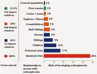
The statistical modelling was based on a
set of numbers – the relative risk of disease to various family members of
people with schizophrenia. Classic studies found that monozygotic twins of schizophrenia
cases had a 48% chance (frequency) of having that diagnosis themselves. For dizygotic
twins, the frequency was 17%. Siblings came in about 10%, half-sibs about 6%,
first cousins about 2%. These figures compare with the population frequency of
~1%.
The statistical modelling inferred that
this pattern of risk, which decreases at a faster than linear pace with respect
to the degree of genetic relatedness, was inconsistent with the condition
arising due to single mutations. By contrast, these data were shown to be
consistent with an oligogenic or polygenic architecture in affected
individuals.
There was however, a crucial (and rather
weird) assumption – that singly causal mutations would all have a dominant mode of inheritance. Under that model, risk would decrease linearly with distance of
relatedness, as it would be just one copy of the mutation being inherited. This
contrasts with recessive modes requiring inheritance of two copies of the
mutation, where risk to distant relatives drops dramatically. There was also an
important assumption of negligible contribution from de novo mutations. As it
happens, it is trivial to come up with some division of cases into dominant,
recessive and de novo modes of inheritance that collectively generate a pattern
of relative risks similar to observed. (Examples of all such modes of
inheritance have now been identified). Indeed, there is an infinite number of ways to set the (many) relevant parameters in order to generate the observed
distribution of relative risks. It is impossible to infer backwards what the
actual parameters are. Not merely difficult or tricky or complex – impossible.
Despite these limitations, these papers
became hugely influential. The conclusion – that schizophrenia could not be caused by mutations in
(many different) single genes – became taken as a proven fact in the field. The
corollary – that it must be caused instead by combinations of common variants –
was similarly embraced as having been conclusively demonstrated.
This highlights an interesting but also
troubling cultural aspect of science – that some claims are based on
methodology that many of the people in the field cannot evaluate. This is
especially true for highly mathematical methods, which most biologists and
psychiatrists are ill equipped to judge. If the authors of such claims are
generally respected then many people will be happy to take them at their word.
In this case, these papers were highly cited, spreading the message beyond
those who actually read the papers in any detail.
In retrospect, these conclusions are
fatally undermined not by the mathematics of the models themselves but by the
simplistic assumptions on which they are based. With that precedent in mind,
let’s return to the GCTA analyses and the strong claims derived from them.
Before considering how the statistical
modelling works (I don’t know) and the assumptions underlying it (we’ll discuss
these), it’s worth asking what the raw findings actually look like.
While the numbers are not provided in this
paper (not even in the extensive supplemental information), we can look at
similar data from a study by the same authors, using cohorts for several other
diseases (Crohn’s disease, bipolar disorder and type 1 diabetes).
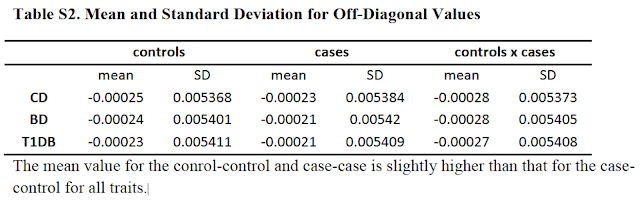
Those numbers are a measure of mean genetic
similarity (i) among cases, (ii) among controls and (iii) between cases and
controls. The important finding is that the mean similarity among cases or
among controls is (very, very slightly) greater than between cases and
controls. All the conclusions rest on this primary finding. Because the sample
sizes are fairly large and especially because all pairwise comparisons are used
to derive these figures, this result is highly statistically significant. But
what does it mean?
The authors remove any persons who are
third cousins or closer, so we are dealing with very distant degrees of genetic
relatedness in our matrix. One problem with looking just at the mean level of
similarity between all pairs is it tells us nothing about the pattern of
relatedness in that sample.
Is the small increase in mean relatedness
driven by an increase in relatedness of just some of the pairs (equivalent to an
excess of fourth or fifth cousins) or is it spread across all of them? Is there
any evidence of clustering of multiple individuals into subpopulations or clans?
Does the similarity represent “identity by descent” or “identity by state”? The
former derives from real genealogical relatedness while the latter could signal
genetic similarity due to chance inheritance of a similar profile of common
variants – presumably enriched in cases by those variants causing disease.
(That is of course what GWAS look for).
If the genetic similarity represents real,
but distant relatedness, then how is this genetic similarity distributed across
the genome, between any two pairs? The expectation is that it would be present mainly
in just one or two genomic segments that happen to have been passed down to
both people from their distant common ancestor. However, that is likely to
track a slight increase in identity by state as well, due to subtle
population/deep pedigree structure. Graham Coop put it this way in an email to
me: “Pairs
of individuals with subtly higher IBS genome-wide are slightly more related to
each other, and so slightly more likely to share long blocks of IBD.”
If we are really dealing with members of a
huge extended pedigree (with many sub-pedigrees within it) – which is
essentially what the human population is – then increased phenotypic similarity
could in theory be due to either common or rare variants shared between distant
relatives. (They would be different rare variants in different pairs).
So, overall, it’s very unclear (to me at
least) what is driving this tiny increase in mean genetic similarity among
cases. It certainly seems like there is a lot more information in those
matrices of relatedness (or in the data used to generate them) than is actually
used – information that may be very relevant to interpreting what this effect means.
Nevertheless, this figure of slightly
increased mean genetic similarity can be fed into models to extrapolate the
heritability explained – i.e., how much of the genetic effects on
predisposition to this disease can be tracked by that distant relatedness. I
don’t know how this model works, mathematically speaking. But there are a
number of assumptions that go into it that are interesting to consider.
First, the most obvious explanation for an
increased mean genetic similarity among cases is that they are drawn from a
slightly different sub-population than controls. This kind of cryptic
population stratification is impossible to exclude in ascertainment methods and
instead must be mathematically “corrected for”. So, we can ask, is this
correction being applied appropriately? Maybe, maybe not – there certainly is
not universal agreement among the Illuminati on how this kind of correction should
be implemented or how successfully it can account for cryptic stratification.
The usual approach is to apply principal components analysis to look for global trends that differentiate the genetic
profiles of cases and controls and to exclude those effects from the models
interpreting real heritability effects. Lee and colleagues go to great lengths
to assure us that these effects have been controlled for properly, excluding up
to 20 components. Not everyone agrees that these approaches are sufficient,
however.

Another major complication is that the relative
number of cases and controls analysed does not reflect the prevalence of the
disease in the population. In these studies, there were about equal numbers of
each in fact, versus a 1:100 ratio of cases to controls in the general
population for disorders like schizophrenia or autism. Does this skewed
sampling affect the results? One can certainly see how it might. If you are
looking to measure an effect where, say, the fifth cousin of someone with
schizophrenia is very, very slightly more likely to have schizophrenia than an
unrelated person, then ideally you should sample all the people in the
population who are fifth cousins and see how many of them have schizophrenia. (This
effect is expected to be almost negligible, in fact. We already know that even
first cousins have only a modestly increased risk of 2%, from a population
baseline of 1%. So going to fifth cousins, the expected effect size would
likely only be around 1.0-something, if it exists at all).
You’d need to sample an awful lot of people
at that degree of relatedness to detect such an effect, if indeed it exists at
all. GCTA analyses work in the opposite direction, but are still trying to
detect that tiny effect. But if you start with a huge excess of people with
schizophrenia in your sample, then you may be missing all the people with
similar degrees of relatedness who did not develop the disease. This could
certainly bias your impression of the effect of genetic relatedness across this
distance.
Lee and colleagues raise this issue and
spend a good deal of time developing new methods to statistically take it into
account and correct for it. Again, I cannot evaluate whether their methods
really accomplish that goal. Generally speaking, if you have to go to great
lengths to develop a novel statistical correction for some inherent bias in
your data, then some reservations seem warranted.
So, it seems quite possible, in the first
instance, that the signal detected in these analyses is an artefact of cryptic
population substructure or ascertainment. But even if it we take it as real, it
is far from straightforward to divine what it means.
The model used to extrapolate heritability
explained has a number of other assumptions. First, is that all genetic
interactions are additive in nature. [See here for arguments why that is
unlikely to reflect biological reality]. Second, it assumes that the
relationship between genetic relatedness and phenotypic similarity is linear
and can be extrapolated across the entire range of relatedness. At least, all
you are supposedly measuring is the tiny effect at extremely low genetic
relatedness – can this really be extrapolated to effects at close relatedness?
We’ve already seen that this relationship is not linear as you go from twins to
siblings to first cousins – those were the data used to argue for a polygenic
architecture in the first place.
This brings us to the final assumption implicit
in the mathematical modelling – that the observed highly discontinuous
distribution of risk to schizophrenia actually reflects a quantitative trait
that is continuously (and normally) distributed across the whole population. A
little sleight of hand can convert this continuous distribution of “liability”
into a discontinuous distribution of cases and controls, by invoking a
threshold, above which disease arises. While genetic effects are modelled as
exclusively linear on the liability scale, the supposed threshold actually
represents a sudden explosion of epistasis. With 1,000 risk variants you’re
okay, but with say 1,010 or 1,020 you develop disease. That’s non-linearity for
free and I’m not buying it.
I also don’t buy an even more fundamental
assumption – that the diagnostic category we call “schizophrenia” is a unitary
condition that defines a singular and valid biological phenotype with a common
etiology. Of course we know it isn’t – it is a diagnosis of exclusion. It
simply groups patients together based on a similar profile of superficial
symptoms, but does not actually imply they all suffer from the same condition.
It is a place-holder, a catch-all category of convenience until more
information lets us segregate patients by causes. So, the very definition of
cases as a singular phenotypic category is highly questionable.
Okay, that felt good.
But still, having gotten those concerns off
my chest, I am not saying that the conclusions drawn from the GCTA analyses of
disorders like schizophrenia and autism are not valid. As I’ve said repeatedly
here, I am not qualified to evaluate the statistical methodology. I do question
the assumptions that go into them, but perhaps all those reservations can be
addressed. More broadly, I question the easy acceptance in the field of these
results as facts, as opposed to the provisional outcome of arcane statistical
exercises, the validity of which remains to be established.


Very detailed post, showing an impressive grasp of the subject for someone who claims ignorance. However, I think there is a good alternative to blind trust. As you correctly argue, we should require a list of the major assumptions made in any statistical model. Then (brace yourself) we should all brush up on our statistics as far as we can. I have some knowledge of statistics, but I lack the higher maths which would make me into a proper commentator. When I read genetic studies, I usually find that the variance accounted for in the replication is reassuringly low, typically 1-3% for general intelligence. When it gets higher I will try to be more critical. Thanks for your post
ReplyDeleteThis comment has been removed by a blog administrator.
ReplyDeleteThanks for a great post, Kevin, I had the same concerns but could not articulate them so elegantly.
ReplyDeleteWe don't know any actual genes with schizophrenia-predisposing recessive variants, right? Were you referring to families that fit the recessive inheritance pattern, or have I missed something?
Yes, you're right, for schizophrenia - no specific genes identified yet with that pattern, but multiple families, plus evidence from patterns of homozygosity (and increased risk with inbreeding):
Deletehttp://www.ncbi.nlm.nih.gov/pubmed/18449909
http://www.ncbi.nlm.nih.gov/pubmed/22511889
http://www.ncbi.nlm.nih.gov/pubmed/23247082
http://www.ncbi.nlm.nih.gov/pubmed/?term=18621663
Great post. I better understand your concerns about applying mixed models to disease. Your Genome Biology paper looks interesting. I think your comments about defining phenotypes is spot on.
ReplyDeleteLee et al did not compare the similarity among cases to the similarity among controls. They fit the phenotype of 0 and 1 as the dependent variable. The linear model estimates an effect for each SNP (u in Efficient methods to compute genomic predictions) and the allele substitution effects of all of the SNPs are summed to estimate the genetic value (a.k.a. breeding value). The SNPs could then account for a certain portion of the variance in 0's and 1's (heritability on the observed scale of an ascertained sample). They then used a formula accounting for the ascertainment of cases and the covariance between observed heritability and liability heritability to estimate the liability heritability (Equation 23 in Estimating Missing Heritability for Disease from Genome-wide Association Studies )
I'm not sure that's right. At least, they say they compute the mean similarity among cases and among controls (and between them) and they say that the crucial observation is that that similarity is higher among cases (as in Table S2). Are you saying it's not just those numbers that are fed into the models, but the entire matrix? That would make more sense, I suppose. The ultimate point is the same though - the conclusions rest on being able to detect a teeny-weeny putative signal of increased risk at distant relatedness to someone with SZ (inverted in the GCTA design, but that's still the supposed effect driving such a signal). So, they have to (i) detect such a signal amidst all the noise and (ii) extrapolate the meaning of such a signal through statistical simulations with various assumptions and methodological complexities.
DeleteHi Kevin,
ReplyDeleteSo the method does not assume that "all genetic interactions are additive in nature" it is trying to estimate the additive genetic variance and the narrow sense heritability (in this case ascribable to common polymorphisms). This is not the same as ignoring interactions, it is simply asking for the additive contribution of each SNP.
Jared is right that they are allowing each locus to have an effect and then computing the variance explained from that. That is equivalent on a conceptual level to examining the relatedness between individuals with similar phenotypes. However, it does not require them to have a sample which is representative of the population in its frequency of cases.
Graham Coop
Yes, fair enough on the additive point - you've worded it more correctly.
DeleteI disagree on the second point - however they implement it, their primary result, on which everything else is based, is increased genetic similarity among cases. At least, that is how the authors themselves describe it. Also, they go to great lengths to "correct for" a skewed sampling that does not reflect population prevalence so it seems it is a genuine problem.
For GCTA, the GWAS data is used to calculate the genetic relationship matrix (GRM) which is used on a linear mixed model which is equivalent to that previously used by quantitative genetics research. The fact that the variance explained by the genetic relationships (capture on the GRM) is > 0 IMPLIES the genetic distance patterns you commented above. But the analysis is done (as in GCTA) based on the GRM, not imputing the distance values.
DeleteThere are studies comparing the results obtained from GCTA analysis to that of twins and show agreement. Consider that GCTA excludes first degree relatives. These two analysis rest on different assumptions (see review linked at the bottom for more on this).
There are also articles describing the link between the model used on GCTA and the equivalent model of fitting a regression with all SNPs simultaneously, they two models are equivalent. So GCTA is equivalent to doing a GWAS with all SNPs together, getting the individual coefficients and using that to make phenotypic predictions. These only captures the additive genetic effects. See this article which discusses estimating dominant effects http://www.genetics.org/content/early/2013/10/07/genetics.113.155176.short . Which is quite interesting I think. There is also a model called single-step Genomic Selection, which combines the GRM with the genetic matrix obtained from pedigrees, so you can obtain h2 estimates with individuals that have been genotyped and those that have not been genotyped. This model seems to be better than pedigree alone (better estimates of genetic relationship) and that using the GRM alone (larger sample size).
The literature on breeding is full of example comparing results from family studies with those obtained with GWAS data on the same samples, the estimate agree well and those from GWAS data are consistently more accurate.
Overall this articles by M Goddard and P Visscher are good introductions to this topic
http://www.annualreviews.org/doi/pdf/10.1146/annurev-animal-031412-103705
http://www.annualreviews.org/doi/pdf/10.1146/annurev-genet-111212-133258
Thanks for those comments, which are very helpful. I have clearly made a mistake in describing the way the analysis is carried out - all the info in the matrix is def into the model, rather than just the mean relatedness.
DeleteHowever, the concept is the same, I think - the result is still driven by that increased mean relatedness - that is the basis for inferring heritability across distant degrees of relatedness. And the magnitude of that effect (across the whole matrix) is extrapolated through the rather complex corrections and simulations to derive an estimate of the amount of variance tagged by common SNPs.
I think the second part is not accurate. I do not think there is any extrapolation neither simulations going on.
DeleteThe methods are the same used by other quantitative genetic analyses. The review by P Visscher linked above shows that is nice and quite readable manner. In one way of another all happening here is estimating the slope of the regression between genetic similarity and phenotypic similarity. As far as it is a linear relationship, (yes that is an assumption but a testable one), one should be able to estimate the slope using values on any range of the data. Twin studies use genetic similarities of 0.5 or 1, other family studies from 1 to something lower (e.g., 0.125 for cousins) and GCTA uses genetic similarity values smaller that any of those. the GRM GCTA uses has lower variance than that of family studies which means it needs more samples go achieve power. BUT GCTA should not be confounded by shared environmental factors neither by dominance (I far as I can see). The last two can be important caveats of h2 estimates from family studies, so GCTA lets you get a h2 estimate free of those confounders.
Same question, what is the h2, same(ish) stats to get the answer but a different kind of data. Nobody is on the dark side of the force as far as I can see :)
I think if you go over that paper the whole thing may become clearer.
I get the idea (I think). But there are assumptions and complex statistical corrections and transformations that go on that extrapolate (or convert, if you prefer), the observed differences in relatedness in the matrix to a value of heritability tagged by all the common SNPs.
DeleteAnd as for the assumption of linearity, there are good reasons to expect MUCH bigger effects at closer degrees of relatedness, if rare variants (under -ve selection) play an important role and if de novo mutation replenishes them in the population. So there seems to me to be a circular logic to that assumption - only valid if the theory these results are supposed to validate is valid.
That biologists (medical doctors included on the category) accept claims from "authorities" on the field without evaluating the basis rigorously is worrying but nothing new under the sun. That biologists are quite ignorant on stats and maths is a serious issue I would say. But it is not the case for all of biology, those working on breeding probably know a fair bit of stats and in my experience it is easier to find ecologist than molecular biologist with good stats knowledge. I think, this is because other branches of biology had the need for more stats training and hands on work before just as physic did before biology.
ReplyDeleteHopefully, things like widespread genetic analysis, genomics and imaging data will push training programs to include more programming and statistics as key professional skills.
PS: I am a biologist ... so nothing personal against biologists
Hi
ReplyDeletethe Post seems to be good ir eally gathered lot of information fromt he Post thanks for sharing this awesome Post
Bollywood movies
You don't really emphasize it, but what's fascinating about this approach is that they claim to found most of the missing heritability. I think these may be the papers Inti Pedroso referred to that aren't exactly GCTA, but use a similar method of inferring relatedness: Genome-wide association studies establish that human intelligence is highly heritable and polygenic, Common SNPs explain a large proportion of heritability for human height
ReplyDeleteIn still missing, Eric Turkheimer argues that these results show the tissue of assumptions underlying quantitative genetics and heritability has now been validated. He isn't specific about which assumptions, but if these approaches hold up, then it it ought to really put a spike in the program of the people trying to talk down heritability in order to avoid genetic determinism. In particular, the current argument that heritability is meaningless "because epigenetics". If 40% heritability for height or IQ has been found by purely genetic means, then even if transgenerational epigenetics is involved, the epigenetics are so linked to the DNA that we might as well call them another kind of genetics.
It could be that you're right about a circularity in the bowels of their analysis, but conceptually it seems that the status of additivity is what it has always been in heritability, which is that they "have no need for that hypothesis" of interaction.
continued...
With the liability model, and assumption of additive interaction, my impression of the quantitative genetics approach is to fit the simplest model that explains the data. For quantitative traits, they've tried adding non-additive terms, and mostly aren't impressed with the results. The hubris of fitting a linear model to human behavior is breathtaking, but the observation is that (so far) it's worked pretty well. When the data stop fitting, it's time for a new model.
ReplyDeleteIs a threshold "nonlinearity for free"? Well, it's a model of nonlinearity presumed to be somewhere in the system, and a threshold is the simplest nonlinearity. As to how this could be plausible, the most obvious explanation is (as you've elsewhere observed) the mind is an emergent system with chaotic potentials. Imagine each small additive factor lifts up the attractor basin just a bit until there's no basin left, and you switch to another attractor (illness.)
For additivity, the quantitative genetics people have heard the complaints that insofar as we understand any small scale genetic pathways and mechanisms, we find it's a complex strongly interacting mess. But they're just not seeing that using their methods. I've been reading a bunch of these papers recently, and don't recall exactly where I read it, but one explanation offered is that the genome may have evolved to interact additively so that evolution works. Though they didn't mention it specifically, this is clearest when you look at sexual reproduction.
Sexual reproduction is an embarrassment for selfish gene theory, but if you think about it, it's pretty clear that we wouldn't be here writing blogs if our ancestors hadn't hit on sex, because it allows us to mix and match adaptive mutations. This greatly speeds up evolution. Yet mix is the operative word here. You have to be able to mix two arbitrary genomes with a high odds of producing viable offspring. If you have strongly interacting genes, then there is a big risk that sexual reassortment will be catastrophic. This is reduced a bit if the genes are near each other, but that's just because the interaction isn't actually revealed, so still no strong interaction.
This is additive interaction is a form of modularity Evolution has hit on the idea of modularity (just as engineers have) because it is really hard to design a complex non-modular (highly interactive) system. You tweak this thing over here and something else breaks. This is one reason why we have differentiated tissues and organs with different functions. But a module doesn't have to be spatially contiguous, it only needs to be logically decoupled. This concept of module is a bit different that "massive mental modularity" as advocated by evolutionary psych, though in order for distinct mental capacities like that to evolve, you'd need genetic modularity too.
@robamacl http://humancond.org
Awesome post, man. This has all the good information that I need. Thumbs up, once again!
ReplyDeleteShuvo,
Clipping Path
This is the primary instant even have glimpsed you’re joyous and do harking back to to apprise you – it's truly pleasing to seem at which i'm appreciative for your diligence. whereas if you expected did it at some point of {a terribly|a really|a awfully} very straightforward methodology that may be truly gracious auto title loan for you. whereas over all I terribly not obligatory you and affirmative will comprise for a alallotmentment of mails like this. several specific gratitude most.
ReplyDelete